1. Quick Start

1.1. Starting MSlice

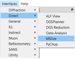
MSlice is included in the Mantid distribution so the easiest way to start it is from the Interfaces menu in MantidWorkbench.

The version of MSlice distributed with Mantid is the last stable version. Starting with MantidWorkbench version 6.12, MSlice is included as a conda package within MantidWorkbench. This enables users to replace the MSlice version within the conda environment where MantidWorkbench is set up. For versions of MantidWorkbench prior to 6.12., it is possible to replace MSlice with the latest development version on GitHub. To get this version, please download this zip and extract it to a folder on your computer. You can then copy the mslice subfolder (the folder containing a file called __init__.py) to the scripts/ExternalInterfaces/ folder of Mantid, which will make the new version accessible from MantidWorkbench.

Alternatively, Mslice is available as a conda package via anaconda.org on the mantid channel. To install the released conda package do mamba install -c mantid mslice. To install the latest nightly conda package do mamba install -c mantid/label/nightly mslice. The nightly conda package includes all recent changes of the development version up to and including the day before and is only created when all tests have run successfully. In both cases MSlice can be started by typing mslice on the command line after activating your conda environment.

When you are using MSlice as an interface in MantidWorkbench, the File menu allows changing the font size of the GUI via the General tab in Settings. Please note that the font size change is only applied after a restart of Mantid. Use Ctrl++ to increase and Ctrl+- to decrease the font size within the Script Editor or the IPython Console.

1.2. Loading Data

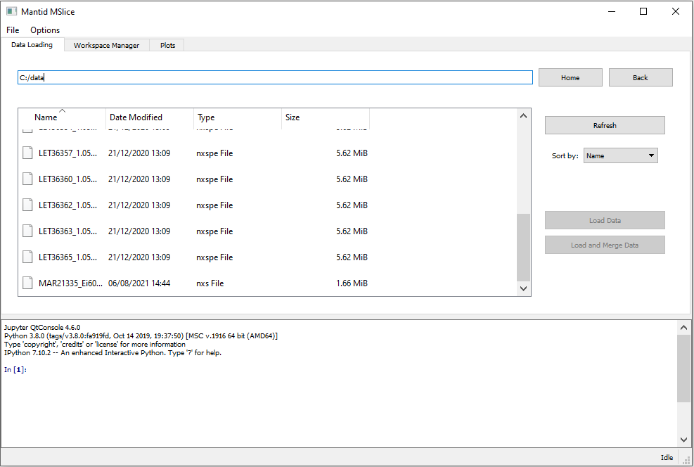
The GUI is divided into three main tabs, a Data Loading tab which shows the filesystem and allows the user to load reduced data files, a Workspace Manager which handles the loaded data, and a Plots tab which provides an easy way to interact with all currently open plots. To reach a particular data folder you can either type the full path to the folder in the edit box, or navigate using the filesystem tree below using either the mouse or keyboard arrow keys and the Enter key, with Backspace used for going up a folder level. Typing the first few letters of a file or folder name will also jump to its location in the tree.

The filesystem tree only shows files which MSlice can load (currently nxs, nxspe and txt or xye files).

Double clicking on a file or pressing Enter when it is selected will load it. You can select multiple files by holding down the Shift key to select a range or the Ctrl key to select individual files. These files may then be loaded separately using the Load Data button or summed together into a single workspace using the Load and Merge Data button. In the later case, the logs of the datafiles are also combined. (Note that you can also sum loaded workspaces together in the Workspace Manager tab after loading, but in this case the logs are not combined).

1.3. PSD and non-PSD modes

Once the data has been loaded, the GUI will switch to the Workspace Manager tab and select the loaded workspace(s). MSlice has two operating modes which it selects automatically depending on the type of data which is loaded. For data from spectrometers with position-sensitive detectors which have been reduced preserving the pixel data (for example, autoreduced data from SNS or one2one mapped data from ISIS), then the PSD mode is used. For these types of data, an extra step to Calculate Projection is required before the data can be plotted. This step converts the data into an MD (multi- dimensional) workspace and then uses the fast binning algorithms for these workspace types which Mantid provides. This step will also be needed for single-crystal data which will be supported in future.

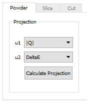
If you have loaded a PSD type dataset, the Slice and Cut tabs will be disabled, and instead a Powder tab will be enabled. Please chose the axes you want to plot (either Momentum Transfer - Energy Transfer, or Scattering Angle - Energy Transfer) and click Calculate Projection. This will create another workspace in the MD Event tab. Selecting it will enable the Slice and Cut tabs to allow you to plot a 2D slice or 1D cut.

On the other hand, if you have loaded a non-PSD type dataset (either from an instrument without position-sensitive detectors or reduced using a rings map), then the Powder tab will be disabled and you can plot a slice or cut directly from the loaded data using the Slice and Cut tabs. In this case, MSlice uses a fractional rebinning algorithm SofQWNormalisedPolygon to directly rebin the powder data.

1.4. Plotting a Slice

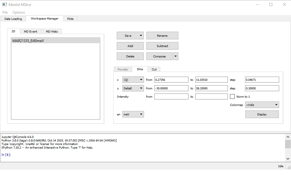
Once the Slice tab is enabled (either directly for loaded non-PSD data, or after calculating projections for PSD data) you can click Display to show a 2D slice of the data. The default values of the limits of the data and step sizes are taken from the input data file. You can change these values and replot. Note that there is a minimum step size which is 1/100 of the default step size which is to ensure that the program does not run out of memory for very small step sizes (which have large number of points). For step sizes smaller than the data step size, some pixels will contain no data and will appear empty (white) in the 2D slice. For more details see Slicing from the GUI.

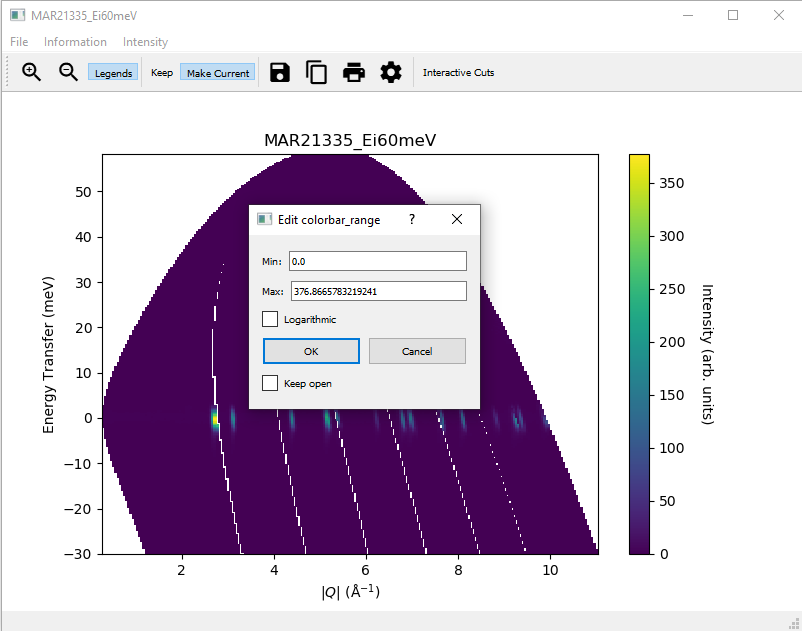
Once the slice is displayed (in a separate window), double clicking on the plot or colorbar axes will allow you to change the plot limits, and whether to use a linear or logarithmic axis. Double clicking on the plot or axes titles will allow you to edit them. Both changing the limits and titles can be done using the options menu accessible from the toolbar.

1.5. Interactive Cuts

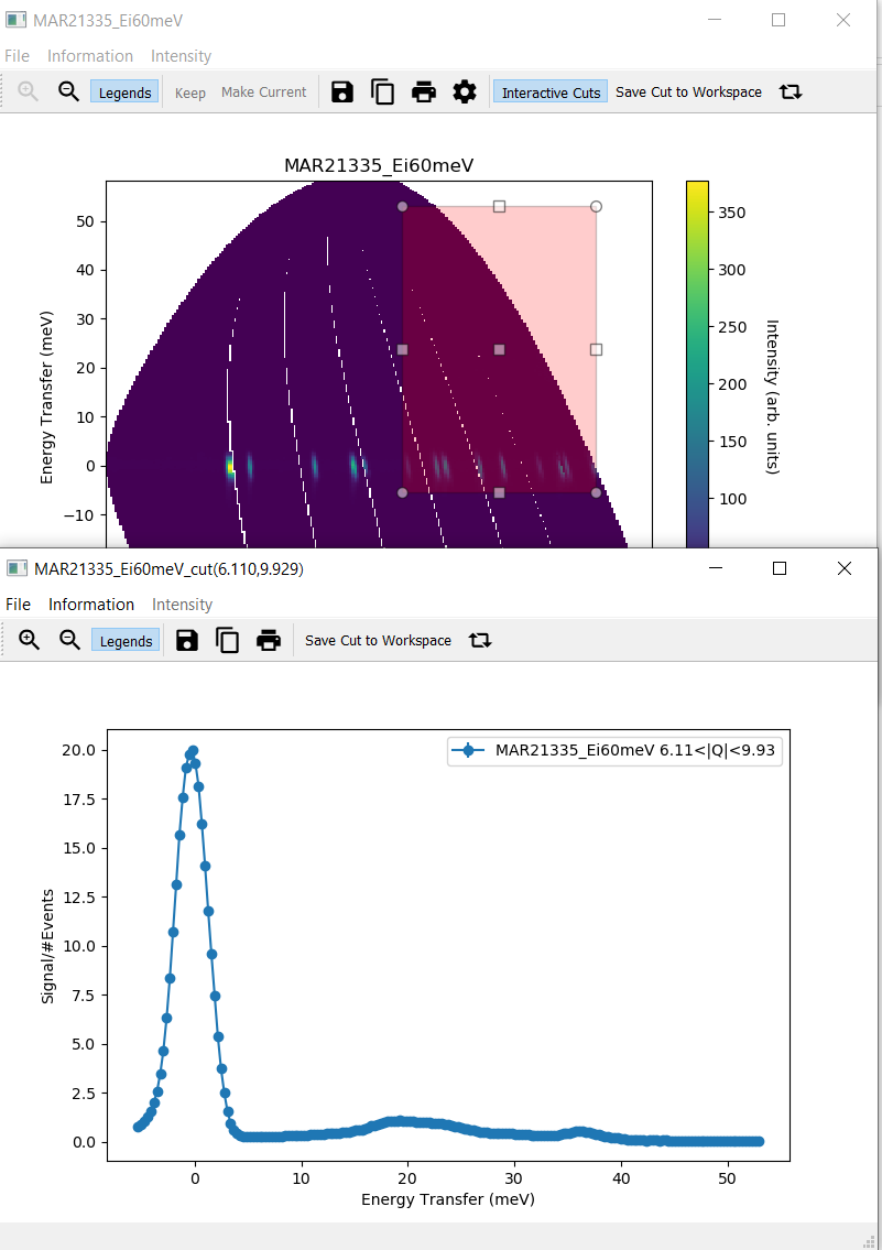
From the slice window, you can also select an Interactive Cut which will allow you to select a region of data to integrate into a 1D and dynamically change this region and the corresponding cut. Clicking Interactive Cut will change the cursor to a cross-hair. You should then select a rectangular region in the 2D slice, after which a separate cut window will open showing the 1D cut. The long axis of the selected rectangle is the cut axis, and the short axis the integration axis. For example, if the 2D plot has Momentum Transfer along x and Energy Transfer along y, selecting a “tall” (vertical) rectangle will result in a cut along Energy Transfer integrating over some region of Momentum Transfer. You can click the rectangular arrows on the toolbar to swap cut and integration axes.

Dragging the rectangle or changing its size in the slice window will update the cut window. You can also redraw the rectangle by clicking outside the current rectangle and dragging. Once you have finished, please click on the Interactive Cut again to leave interactive mode. If you leave a slice in interactive cut mode and plot another slice, another window will open. Making a cut (see below) whilst the interactive mode is active will overplot on the same window as the interactive cut and this cut will be removed when the interactive mode rectangle is moved again. Only when you click Save Cut to Workspace is an MD Histo type workspace created.

1.6. Plotting a Cut

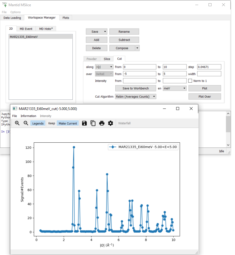
Instead of an interactive cut, you can use the main GUI to specify more specific limits and step sizes for cuts. This will also allow you to overplot multiple cuts from the same dataset with different integration ranges, or from different datasets. To overplot multiple ranges, you can also use the width parameter. This splits in specified integration ranges into chunks of the widths specified. For example, if from is 0 and to is 10 and width is 3, Mslice will plot 4 cuts which integrate over [0,3], [3,6], [6,9] and [9,10] respectively.

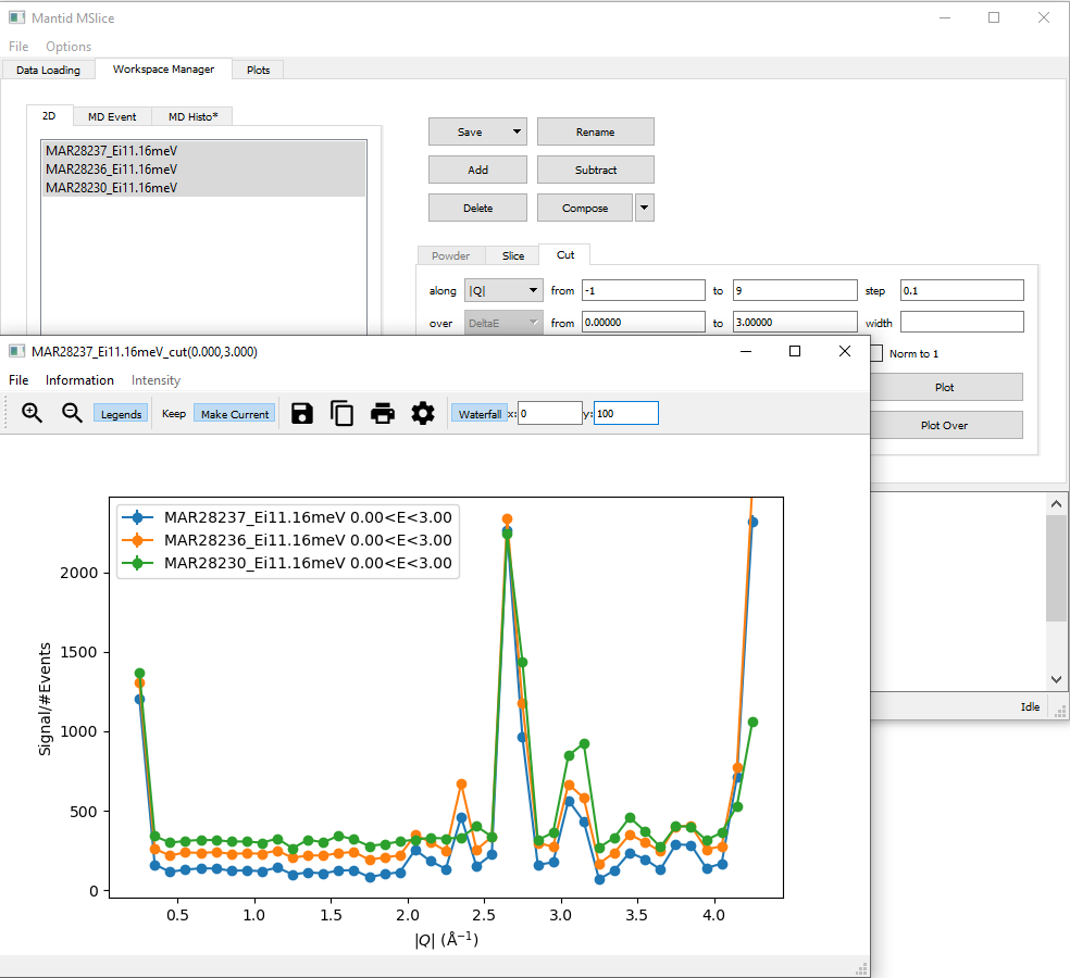
To overplot multiple datasets, you can select multiple workspaces in the left pane (using Shift or Ctrl) and then give common limits, step sizes and integration range, and click Plot. For more details see Cutting from the GUI.

The Waterfall button allows modifying the offsets for the x and y axes when plotting multiple cuts.

1.7. Keep / Make Current

This version of MSlice supports the window management behaviour introduced by the original Matlab MSlice, which is controlled by two buttons, Keep and Make Current, in the toolbar of every plot window. When you click on Display or Plot on the main GUI, the resulting plot will appear in the Current window, over-writing any previous plots in that window. If you want to keep the data in a particular window, click Keep. Subsequent plots will then open a new window. If you subsequently want to overwrite the data on the same particular window, you can make it Current again by clicking Make Current. In order to overplot new data preserving previous data, use the Plot Over button rather than the Plot button. This will send data to the Current plot window, so you may need to Make Current on it again. This is available only for 1D cuts. For 2D slices, you cannot overplot current data.

1.8. Manipulating Workspaces

MSlice supports some basic workspace operations at present and more are planned for future releases. For loaded workspaces, summing and background subtraction are supported, whilst for processed workspaces (MD Event workspaces in PSD mode), only merging workspaces are supported. This is intended primarily for merging HYSPEC data at different detector scattering angles.

In order to sum several workspaces, select multiple workspaces in the workspace panel and click Add. A new workspace named after the first selected workspace with _sum appended will be created.

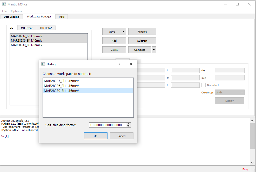
To subtract a background dataset from sample dataset(s), first select one or more sample workspace(s). Then click Subtract. A dialog will appear asking you to select the background dataset to subtract and optionally allow you to specify a self-shielding factor. This self-shielding factor is applied to the background dataset first before it is subtracted from the sample dataset(s). The subtraction is done on each sample workspace individually.

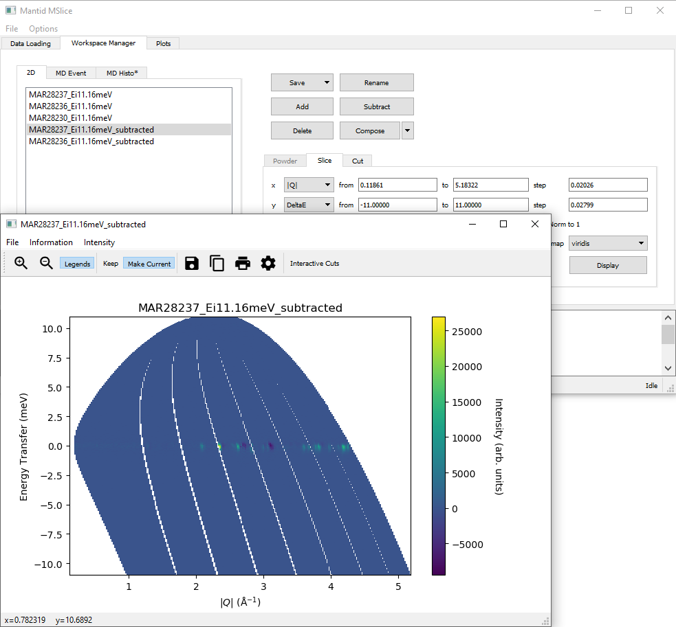
For example, in the image above, two sample workspaces, MAR28237_Ei11.16meV and MAR28236_Ei11.16meV are selected. Then the dataset MAR28230_Ei11.16meV is selected with a self-shielding factor of 1.00. Clicking Ok will produce two subtracted workspaces, MAR28237_Ei10.00meV_subtracted and MAR28236_Ei10.00meV_subtracted. The subtracted dataset can be sliced or cut as usual.

1.9. Energy transfer units

By default MSlice uses meV as the unit for energy transfer, with the convention that positive energy transfer corresponds neutron energy loss. In addition to this, MSlice also supports cm^-1 (wavenumbers), denoted cm-1.

You can choose the desired unit using the en drop-down comboboxes in the Cut and Slice tabs.

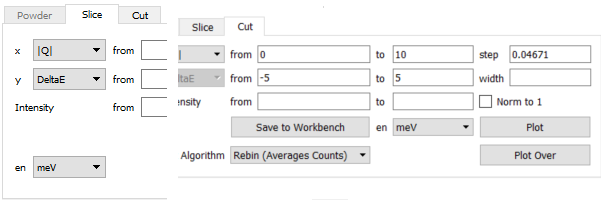
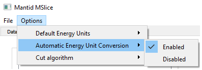
Alternatively you can also set a default energy unit using the Options menu item

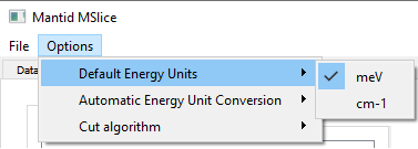
This default energy unit will be applied to Cut and Slice tabs for new workspaces. The cut tab for old workspaces will have the previous energy unit if you’ve made a cut of that workspace before (together with the other parameters of the cut).

Finally, if you first plot a cut using one energy unit (say meV) but then over-plot another energy cut using a different unit (say cm-1), MSlice will automatically convert the previous cuts to the new energy unit (cm-1 in this case), and replot everything in the new unit. If you don’t want this behaviour, you can turn it off in the Options menu: