4. Command Line Interface
4.1. Generating scripts
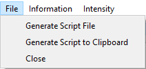
Each MSlice plot window has an option in the File menu to generate a script that would reproduce the plot. This will include the
full history of the workspace which provides the data for the plot, and additionally any graphical changes to the plot above the
default (e.g. if the axes titles or limits have been changed or additional information such as recoil or Bragg lines added). The
script can either be written to a file or copied to the clipboard.
Generated scripts may be run from the MantidWorkbench script window.
Alternatively, when written to a file the script can also be run from the IPython console in the MSlice GUI using the import
directive and the reload (importlib.reload in Python 3) function. For example, the first time the script is run, do:
import script_name
for a script file named script_name.py which is on the Python path. Subsequently, if you change the script file and want to re-run it,
you can do:
reload(script_name)
4.2. Plotting using Matplotlib interface
Whilst MSlice uses Matplotlib to render all the plots, it has its own type of figure windows in order to accommodate additional features such as the keep / make current functionality and interactive plots. The MSlice specific figures do not support multiple plots per figure (subplots) and will not work in a Jupyter notebook. However, MSlice is also able to plot to a generic Matplotlib figure.
To plot a 1D cut using the MSlice figures use:
import mslice.cli as mc
import mslice.plotting.pyplot as plt

ws = mc.Load('data.nxspe')
cut_ws = mc.Cut(ws, '|Q|', 'DeltaE, -1, 1')

fig = plt.figure()
ax = fig.add_subplot(111, projection='mslice')
ax.errorbar(cut_ws, fmt='ok')
ax.set_ylim(0., 0.1)

mc.Show()
To plot the same cut using a plain Matplotlib figure use:
import mslice.cli as mc
import matplotlib.pyplot as plt

ws = mc.Load('data.nxspe')
cut_ws = mc.Cut(ws, '|Q|', 'DeltaE, -1, 1')

fig = plt.figure()
ax = fig.add_subplot(111, projection='mslice')
ax.errorbar(cut_ws, fmt='ok')
ax.set_ylim(0., 0.1)

fig.show()
E.g. the only difference is that you must use the matplotlib.pyplot package instead of the mslice.plotting.pyplot package
and call fig.show() at the end instead of mc.Show(). In both cases, all the standard object-oriented Matplotlib functions
(such as set_title, set_xlabel, set_xlim etc.) are accepted. Note that also in both cases you must specify the
projection='mslice' keyword argument to add_subplot, because this lets the Matplotlib errorbar function recognise an
MSlice workspace. Finally, please also that the MSlice override of pyplot does not support the fig, ax = plt.subplots()
syntax.
You must also use errorbar to plot a 1D cut, and pcolormesh to plot a 2D slice. No other Matplotlib plotting function are
aware of MSlice workspaces (even with the projection='mslice' argument).
An example of plotting a slice:
import mslice.cli as mc
import matplotlib.pyplot as plt

ws = mc.Load('data.nxspe')
slice_ws = mc.Slice(ws, '|Q|, 0, 10, 0.01', 'DeltaE, -5, 55, 0.5')

fig = plt.figure()
ax = fig.add_subplot(111, projection='mslice')
mesh = ax.pcolormesh(slice_ws, cmap='coolwarm')
mesh.set_clim(0, 1)
cb = plt.colorbar(mesh, ax=ax)

fig.show()
4.3. Plotting using MSlice specific commands
In addition to using the Matplotlib-style object-oriented interface (defining a figure and then add_subplot), there are
also MSlice functions which will wrap these commands and plot to an MSlice figure (e.g. does not work in Jupyter, does not support
multiple subplots, but has all the GUI tools (overplot recoil lines / Bragg peaks, interactive cuts, etc.). These commands, whilst
shorter, are not as flexible as the Matplotlib object-oriented interface, however.
To plot a cut and then a slice:
import mslice.cli as mc

ws = mc.Load('data.nxspe')
wsq = mc.Cut(ws, '|Q|', 'DeltaE, -1, 1')
mc.PlotCut(wsq)

ws2d = mc.Slice(ws, '|Q|, 0, 10, 0.01', 'DeltaE, -5, 55, 0.5')
mc.PlotSlice(ws2d)
4.4. Algebraic Manipulation of Workspaces
The MSlice workspaces support standard algebraic manipulations in a similar way to normal Mantid workspaces. Loaded nxs or
nxspe files are created as a Workspace. For PSD (one-to-one mapped) files, these are first converted into a
PixelWorkspace using a “Calculate Projection” step before they can be plotted. The slices and cuts produced either directly
from the loaded Workspace (if in non-PSD mode, e.g. for a rings-mapped file) or from the PixelWorkspace are
HistogramWorkspaces.
Operations performed on Workspacess and HistogramWorkspacess are done per bin, so only operations with a matching sized
workspace, or with a scalar is allowed. For PixelWorkspace (which are based on Mantid’s MDEventWorkspace which does not
allow many algebraic manipulations), a fine grained slice is first created (generating an internal HistogramWorkspace) and
then the algebraic operation is applied to this fine grained slice. Thus it is recommended to perform any algebraic manipulation
on the loaded Workspace prior to conversion (using MakeProjection) to a PixelWorkspace for cutting / slicing and
plotting.
For example:
import mslice.cli as mc

ws1 = mc.Load('data.nxspe')
ws2 = mc.Load('background.nxspe')
ws = ws1 - 0.8 * ws2
mc.PlotSlice(mc.Slice(ws))
4.5. Examples
4.5.1. Loading and Cutting / Slicing
To load and plot a slice in  and energy transfer, and a cut along , integrating over
  :
:
import mslice.cli as mc

ws = mc.Load('data.nxspe')
wsq = mc.Cut(ws, '|Q|', 'DeltaE, -1, 1')
mc.PlotCut(wsq)

ws2d = mc.Slice(ws, '|Q|, 0, 10, 0.01', 'DeltaE, -5, 55, 0.5')
mc.PlotSlice(ws2d)
In the above Slice function rebins the data between  in steps of 0.01
  and between
  in steps of 0.5 meV.
4.5.2. Plotting a series of cuts
import mslice.cli as mc

# Plot a series of energy cuts at different Q (similar to putting something in the width box in GUI).
ws = mc.Load('data.nxspe')
for qq in np.linspace(0.5, 2, 4):
    mc.PlotCut(mc.Cut(ws, 'DeltaE', '|Q|, %f, %f' % (qq-0.5, qq+0.5)), PlotOver=True)

# Loads a series of datasets at different temperatures and plots the energy cuts at low energy
runs = range(103154, 103158)
wss = []
for rr in runs:
    wss.append(mc.Load('SEQ_%06d_powder.nxspe' % (rr)))
    mc.PlotCut(mc.Cut(wss[-1], 'DeltaE', '|Q|, 0, 2'), PlotOver=True)
4.5.3. Saving a series of cuts
import mslice.cli as mc

# Save a series of energy cuts at different Q (similar to putting something in the width box in GUI).
ws = mc.Load('data.nxspe')
for qq in np.linspace(0.5, 2, 4):
    cutws = mc.Cut(ws, 'DeltaE', '|Q|, %f, %f' % (qq-0.5, qq+0.5))
    mc.save_ascii(cutws, '/home/user/'+cutws.name)