StartLiveData v1#

Summary#

Begin live data monitoring.

Properties#

Name	Direction	Type	Default	Description
FromNow	Input	boolean	True	Process live data starting from the current time only.
FromStartOfRun	Input	boolean	False	Record live data, but go back to the start of the run and process all data since then.
FromTime	Input	boolean	False	Record live data, but go back to a specific time and process all data since then. You must specify the StartTime property if this is checked.
UpdateEvery	Input	number	30	Frequency of updates, in seconds. Default 30. If you specify 0, MonitorLiveData will not launch and you will get only one chunk.
Instrument	Input	string	Mandatory	Name of the instrument to monitor.
Connection	Input	string		Selects the listener connection entry to use. Default connection will be used if not specified
Listener	Input	string		Name of the listener class to use. If specified, overrides class specified by Connection. Allowed values: [‘FakeEventDataListener’, ‘FileEventDataListener’, ‘ISISHistoDataListener’, ‘ISISLiveEventDataListener’, ‘KafkaEventListener’, ‘KafkaHistoListener’, ‘SINQHMListener’, ‘SNSLiveEventDataListener’, ‘’]
Address	Input	string		Address for the listener to connect to. If specified, overrides address specified by Connection.
StartTime	Input	string		Absolute start time, if you selected FromTime. Specify the date/time in UTC time, in ISO8601 format, e.g. 2010-09-14T04:20:12.95
ProcessingAlgorithm	Input	string		Name of the algorithm that will be run to process each chunk of data. Optional. If blank, no processing will occur.
ProcessingProperties	Input	string		The properties to pass to the ProcessingAlgorithm, as a single string. The format is propName=value;propName=value
ProcessingScript	Input	string		A Python script that will be run to process each chunk of data. Only for command line usage, does not appear on the user interface.
ProcessingScriptFilename	Input	string		A Python script that will be run to process each chunk of data. Only for command line usage, does not appear on the user interface. Allowed values: [‘py’]
AccumulationMethod	Input	string	Add	Method to use for accumulating each chunk of live data. - Add: the processed chunk will be summed to the previous outpu (default). - Replace: the processed chunk will replace the previous output. - Append: the spectra of the chunk will be appended to the output workspace, increasing its size. Allowed values: [‘Add’, ‘Replace’, ‘Append’]
PreserveEvents	Input	boolean	False	Preserve events after performing the Processing step. Default False. This only applies if the ProcessingAlgorithm produces an EventWorkspace. It is strongly recommended to keep this unchecked, because preserving events may cause significant slowdowns when the run becomes large!
PostProcessingAlgorithm	Input	string		Name of the algorithm that will be run to process the accumulated data. Optional. If blank, no post-processing will occur.
PostProcessingProperties	Input	string		The properties to pass to the PostProcessingAlgorithm, as a single string. The format is propName=value;propName=value
PostProcessingScript	Input	string		A Python script that will be run to process the accumulated data.
PostProcessingScriptFilename	Input	string		Python script that will be run to process the accumulated data. Allowed values: [‘py’]
RunTransitionBehavior	Input	string	Restart	What to do at run start/end boundaries? - Restart: the previously accumulated data is discarded. - Stop: live data monitoring ends. - Rename: the previous workspaces are renamed, and monitoring continues with cleared ones. Allowed values: [‘Restart’, ‘Stop’, ‘Rename’]
AccumulationWorkspace	Output	Workspace		Optional, unless performing PostProcessing: Give the name of the intermediate, accumulation workspace. This is the workspace after accumulation but before post-processing steps.
OutputWorkspace	Output	Workspace	Mandatory	Name of the processed output workspace.
LastTimeStamp	Output	string		The time stamp of the last event, frame or pulse recorded. Date/time is in UTC time, in ISO8601 format, e.g. 2010-09-14T04:20:12.95
MonitorLiveData	Output	IAlgorithm		A handle to the MonitorLiveData algorithm instance that continues to read live data after this algorithm completes.

Description#

The StartLiveData algorithm launches a background job that monitors and processes live data.

The background algorithm started is MonitorLiveData v1, which simply calls LoadLiveData v1 at a fixed interval.

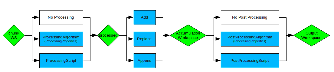
Live data processing workflow showing how data flows through processing and accumulation steps#

Note

For details on the way to specify the data processing steps, see LoadLiveData.

Instructions for setting up a “fake” data stream are found here.

Listener Properties#

Specific LiveListeners may provide their own properties, in addition to properties provided by StartLiveData. For convenience and accessibility, these properties are made available through StartLiveData as well.

In the StartLiveData algorithm dialog, a group box called “Listener Properties” will appear at the bottom of the sidebar on the left, if the currently selected listener provides additional properties.

In the Python API, these listener properties may also be set as keyword arguments when calling StartLiveData. For example, in this code snippet:

StartLiveData(Instrument='ISIS_Histogram', OutputWorkspace='wsOut', UpdateEvery=1,
              AccumulationMethod='Replace', PeriodList=[1,3], SpectraList=[2,4,6])

PeriodList and SpectraList are properties of the ISISHistoDataListener. They are available as arguments in this call because Instrument is set to ‘ISIS_Histogram’, which uses that listener.

KafkaEventListener#

BufferThreshold defines the number of events (default 1000000) to hold in the intermediate buffer before it is flushed to the streamed EventWorkspace. This parameter must be tuned to the data you are streaming. Setting this parameter too high for your event rate will cause behaviour that make live streaming appear to have stalled. Setting this too low may cause performance issues with high count rates.

There is no general rule for deriving this parameter that will give the best performance. To ensure that live streaming remains responsive this parameter should be set to UpdateEvery times the approximate event rate. Due to the nature of the intermediate buffer it is not possible to avoid having to know the approximate event rate before streaming.

25000000 has shown to work well for simulated LOKI data at 10e7 events per second.

Live Plots#

Once live data monitoring has started, you can open a plot and as the data is acquired, this plot updates automatically.

StartLiveData algorithm returns after the first chunk of data has been loaded and processed. This makes it simple to write a script that will open a live plot. For example:

StartLiveData(UpdateEvery='1.0',Instrument='FakeEventDataListener',
  ProcessingAlgorithm='Rebin',ProcessingProperties='Params=10e3,1000,60e3;PreserveEvents=1',
  OutputWorkspace='live')
plotSpectrum('live', [0,1])

Interactive Usage Guide#

This section provides practical guidance for using StartLiveData interactively in Mantid Workbench to monitor experiments in real-time.

Getting Started#

Prerequisites:

Mantid Workbench installed
Network access to the instrument’s Data Acquisition System (DAS)
Facility and instrument configured in Mantid settings

Quick Start Steps:

Configure Mantid settings - Open Workbench: File → Settings. Set Facility (e.g., “SNS” or “ISIS”) and Default Instrument (e.g., “POWGEN”, “REF_M”)
Open StartLiveData - Click the algorithm search or press Ctrl+F, type “StartLiveData” and open it

Configure basic properties:

Instrument: (auto-filled from settings)
UpdateEvery: 30  # seconds between updates
OutputWorkspace: live_data

Set timing options - Choose from:
- From Start of Run: Collect all data since run began (recommended)
- From Now: Only collect data from this moment forward
- From Time: Start from specific timestamp
Configure processing (optional) - Processing tab: Add algorithms to run on each chunk. Example: Use “Rebin” with Params=”1000,100,20000”
Configure post-processing (optional) - Post-Processing Step tab: Select “Python Script” and load your post-processing script, or choose an algorithm to run on accumulated data
Click “Run” to start live data collection
Monitor the data - Right-click the live_data workspace → Plot Spectrum. The plot updates automatically as data arrives. Check the Messages panel for errors
Stop collection - Click the “Details” button (bottom right of Workbench), then click “Cancel” next to MonitorLiveData

Simple Monitoring Examples#

Basic Monitoring#

For quick visualization without custom processing:

# In Workbench's script window or Python interface
from mantid.simpleapi import StartLiveData

StartLiveData(
    Instrument='POWGEN',
    OutputWorkspace='monitor',
    UpdateEvery=30,
    FromStartOfRun=True,
    AccumulationMethod='Add'
)

# Now plot it
plotSpectrum('monitor', [0, 1, 2])

The plot updates automatically as new data arrives.

Use cases:

Checking if the instrument is collecting data
Monitoring detector health
Quick visualization during alignment
Verifying event rates
Sanity checking during setup

With Processing Algorithm#

Apply reduction during acquisition:

from mantid.simpleapi import StartLiveData

StartLiveData(
    Instrument='NOMAD',
    UpdateEvery=60,
    AccumulationMethod='Add',
    ProcessingAlgorithm='AlignAndFocusPowder',
    ProcessingProperties='CalFilename=/SNS/NOM/shared/CALIBRATION.cal;'
                        'GroupFilename=/SNS/NOM/shared/GROUP.xml',
    AccumulationWorkspace='accumulated',
    OutputWorkspace='live_nomad'
)

What happens:

Every 60s, new chunk arrives
AlignAndFocusPowder processes it
Result added to accumulated
live_nomad shows current accumulated state

Starting from Specific Time#

Resume monitoring from earlier in the run:

from mantid.simpleapi import StartLiveData
from datetime import datetime, timedelta

# Start from 5 minutes ago
start_time = datetime.now() - timedelta(minutes=5)

StartLiveData(
    Instrument='CORELLI',
    FromTime=start_time.strftime('%Y-%m-%dT%H:%M:%S'),
    UpdateEvery=30,
    OutputWorkspace='live_corelli'
)

Use cases:

Catch up after Workbench restart
Review recent data while run continues
Compare different time windows

Custom Processing with Python Script#

Use external processing script for complex workflows.

Create my_reduction.py:

from mantid.simpleapi import (
    ConvertUnits,
    Rebin,
    SumSpectra,
    SaveNexus
)

# Process chunk
ConvertUnits(
    InputWorkspace=input,
    OutputWorkspace=output,
    Target='dSpacing'
)

Rebin(
    InputWorkspace=output,
    OutputWorkspace=output,
    Params='0.5,0.01,3.5',
    PreserveEvents=False
)

# Sum for quick view
SumSpectra(
    InputWorkspace=output,
    OutputWorkspace='summed',
    RemoveSpecialValues=True
)

# Optional: Save each chunk
run_number = output.getRun().getProperty('run_number').value
SaveNexus(
    InputWorkspace=output,
    Filename=f'/SNS/POWGEN/IPTS-12345/shared/live_chunk_{run_number}.nxs'
)

Run with script:

StartLiveData(
    Instrument='POWGEN',
    UpdateEvery=45,
    ProcessingScriptFilename='/path/to/my_reduction.py',
    AccumulationMethod='Add',
    OutputWorkspace='live_reduced'
)

Understanding Timing Options#

The timing options control what data you receive when connecting:

FromStartOfRun (Recommended)#

What it does: Collects all data since the current run began

When to use: Starting monitoring mid-run, want complete picture

How it works:

DAS buffers all events/histograms since run start
You receive everything collected so far
Then continues with new data as it arrives

FromNow#

What it does: Only collects data from the moment you connect

When to use: Only interested in future data, memory constrained

Trade-offs:

Misses anything collected before connection
Lower memory usage
Simpler for quick checks

FromTime#

What it does: Starts collecting from a specific timestamp

Format: UTC, ISO8601 format (e.g., “2026-01-21T14:30:00”)

When to use: Replaying or analyzing specific time windows

UpdateEvery#

What it does: How often (in seconds) post-processing runs

Default: 30 seconds

Trade-offs:

Shorter = more responsive but more CPU usage
Longer = less overhead but slower updates
Does not affect how often chunks arrive (DAS controls that)

Practical Example Scenarios#

Monitoring Detector Health#

StartLiveData(
    Instrument='NOMAD',
    OutputWorkspace='detector_check',
    UpdateEvery=10,
    FromNow=True,
    AccumulationMethod='Replace'
)
# Plot updates every 10 seconds with latest data only

Accumulating Full Run Data#

StartLiveData(
    Instrument='POWGEN',
    OutputWorkspace='full_run',
    UpdateEvery=30,
    FromStartOfRun=True,
    AccumulationMethod='Add',
    PreserveEvents=False  # Convert to histogram to save memory
)

Time-Series Analysis#

StartLiveData(
    Instrument='CORELLI',
    OutputWorkspace='timeseries',
    UpdateEvery=60,
    FromStartOfRun=True,
    AccumulationMethod='Append'  # Each chunk becomes separate spectrum
)

Common Issues and Troubleshooting#

Connection Fails#

Symptoms: Cannot connect to live data stream

Check:

Network access to DAS
Facility/instrument settings correct
Instrument is actually running
Firewall settings allow connection

Memory Fills Up#

Symptoms: Mantid becomes slow or crashes during live monitoring

Solutions:

Set PreserveEvents=False to convert to histograms
Use AccumulationMethod='Replace' instead of ‘Add’
Increase UpdateEvery to reduce frequency
Close other memory-intensive applications
Use CompressEvents in post-processing for event data

Plot Doesn’t Update#

Symptoms: Workspace exists but plot is static

Check:

MonitorLiveData is still running (check Details button)
Log messages for errors
DAS is sending data (ask instrument scientist)
Plot window is set to auto-refresh

Data Processing Errors#

Symptoms: Errors in processing or post-processing steps

Debug steps:

Test processing algorithm separately with static data
Check algorithm property syntax in ProcessingProperties
Review python script for syntax errors
Verify file paths and calibration files exist
Check log messages for specific error details

Tips for Interactive Use#

Start with FromStartOfRun=True to get all existing data
Use UpdateEvery=10 for faster updates during testing
Watch memory usage in system monitor when preserving events
Test scripts with fake data servers (see Live Data Testing)
Use the algorithm dialog to build property strings, then copy to scripts

Run Transition Behavior#

When the experimenter starts and stops a run, the Live Data Listener receives this as a signal.
The RunTransitionBehavior property specifies what to do at these run transitions.
- Restart: the accumulated data (from the previous run if a run has just ended or from the time between runs a if a run has just started) is discarded as soon as the next chunk of data arrives.
- Stop: live data monitoring ends. It will have to be restarted manually.
- Rename: the previous workspaces are renamed, and monitoring continues with cleared ones. The run number, if found, is used to rename the old workspaces.
  - There is a check for available memory before renaming; if there is not enough memory, the old data is discarded.
Note that LiveData continues monitoring even if outside of a run (i.e. before a run begins you will still receive live data).

Multiple Live Data Sessions#

It is possible to have multiple live data sessions running at the same time. Simply call StartLiveData more than once, but make sure to specify unique names for the OutputWorkspace.

Please note that you may be limited in how much simultaneous processing you can do by your available memory and CPUs.

Usage#

Example 1:

from threading import Thread
import time

def startFakeDAE():
    # This will generate 2000 events roughly every 20ms, so about 50,000 events/sec
    # They will be randomly shared across the 100 spectra
    # and have a time of flight between 10,000 and 20,000
    try:
        FakeISISEventDAE(NPeriods=1,NSpectra=100,Rate=20,NEvents=1000)
    except RuntimeError:
        pass

def captureLive():
    ConfigService.setFacility("TEST_LIVE")

    try:
        # start a Live data listener updating every second, that rebins the data
        # and replaces the results each time with those of the last second.
        StartLiveData(Instrument='ISIS_Event', OutputWorkspace='wsOut', UpdateEvery=1,
                      ProcessingAlgorithm='Rebin', ProcessingProperties='Params=10000,1000,20000;PreserveEvents=1',
                      AccumulationMethod='Add', PreserveEvents=True)

        # give it a couple of seconds before stopping it
        time.sleep(2)
    finally:
        # This will cancel both algorithms
        # you can do the same in the GUI
        # by clicking on the details button on the bottom right
        AlgorithmManager.cancelAll()
        time.sleep(1)
#--------------------------------------------------------------------------------------------------

oldFacility = ConfigService.getFacility().name()
thread = Thread(target = startFakeDAE)

try:
    thread.start()
    time.sleep(2) # give it a small amount of time to get ready
    if not thread.is_alive():
        raise RuntimeError("Unable to start FakeDAE")
    captureLive()
except Exception as e:
    print(f"Error occurred starting live data: {str(e)}")
finally:
    thread.join() # this must get hit

# put back the facility
ConfigService.setFacility(oldFacility)

#get the output workspace
wsOut = mtd["wsOut"]
print("The workspace contains %i events" % wsOut.getNumberEvents())

Output:

 The workspace contains ... events

Example 2:

from threading import Thread
import time

def startFakeDAE():
    # This will generate 5 periods of histogram data, 10 spectra in each period,
    # 100 bins in each spectrum
    try:
        FakeISISHistoDAE(NPeriods=5,NSpectra=10,NBins=100)
    except RuntimeError:
        pass

def captureLive():
    ConfigService.setFacility("TEST_LIVE")

    try:
        # Start a Live data listener updating every second,
        # that replaces the results each time with those of the last second.
        # Load only spectra 2,4, and 6 from periods 1 and 3
        StartLiveData(Instrument='ISIS_Histogram', OutputWorkspace='wsOut', UpdateEvery=1,
                      AccumulationMethod='Replace', PeriodList=[1,3],SpectraList=[2,4,6])

        # give it a couple of seconds before stopping it
        time.sleep(2)
    finally:
        # This will cancel both algorithms
        # you can do the same in the GUI
        # by clicking on the details button on the bottom right
        AlgorithmManager.cancelAll()
        time.sleep(1)
#--------------------------------------------------------------------------------------------------

oldFacility = ConfigService.getFacility().name()
thread = Thread(target = startFakeDAE)

try:
    thread.start()
    time.sleep(2) # give it a small amount of time to get ready
    if not thread.is_alive():
        raise RuntimeError("Unable to start FakeDAE")
    captureLive()
except Exception as e:
    print(f"Error occurred starting live data: {str(e)}")
finally:
    thread.join() # this must get hit

# put back the facility
ConfigService.setFacility(oldFacility)

#get the output workspace
wsOut = mtd["wsOut"]
print("The workspace contains %i periods" % wsOut.getNumberOfEntries())
print("Each period   contains %i spectra" % wsOut.getItem(0).getNumberHistograms())
time.sleep(1)

Output:

 The workspace contains ... periods
 Each period   contains ... spectra

Source#

C++ header: StartLiveData.h

C++ source: StartLiveData.cpp

StartLiveData v1#

Summary#

See Also#

Properties#

Description#

Listener Properties#

KafkaEventListener#

Live Plots#

Interactive Usage Guide#

Getting Started#

Simple Monitoring Examples#

Basic Monitoring#

With Processing Algorithm#

Starting from Specific Time#

Custom Processing with Python Script#

Understanding Timing Options#

FromStartOfRun (Recommended)#

FromNow#

FromTime#

UpdateEvery#

Practical Example Scenarios#

Monitoring Detector Health#

Accumulating Full Run Data#

Time-Series Analysis#

Common Issues and Troubleshooting#

Connection Fails#

Memory Fills Up#

Plot Doesn’t Update#

Data Processing Errors#

Tips for Interactive Use#

Run Transition Behavior#

Multiple Live Data Sessions#

Usage#

Source#

This Page

StartLiveData v1#

Summary#

See Also#

Properties#

Description#

Listener Properties#

KafkaEventListener#

Live Plots#

Interactive Usage Guide#

Getting Started#

Simple Monitoring Examples#

Basic Monitoring#

With Processing Algorithm#

Starting from Specific Time#

Custom Processing with Python Script#

Understanding Timing Options#

FromStartOfRun (Recommended)#

FromNow#

FromTime#

UpdateEvery#

Practical Example Scenarios#

Monitoring Detector Health#

Accumulating Full Run Data#

Time-Series Analysis#

Common Issues and Troubleshooting#

Connection Fails#

Memory Fills Up#

Plot Doesn’t Update#

Data Processing Errors#

Tips for Interactive Use#

Run Transition Behavior#

Multiple Live Data Sessions#

Usage#

Related Resources#

Source#

This Page